A complete 16-channel MCA for SDD and transistor-reset detectors on the x5560 family

Introduction

Silicon Drift Detectors (SDD) and other low-capacitance X-ray detectors are usually read out by transistor-reset (pulsed-reset) charge preamplifiers: instead of a continuous discharge through a feedback resistor, the integrator output ramps up with the detector leakage current and with every absorbed photon, until a reset transistor brings it back to the starting level. The output waveform is a staircase: small steps are photons, the periodic fast falling edge is the reset.

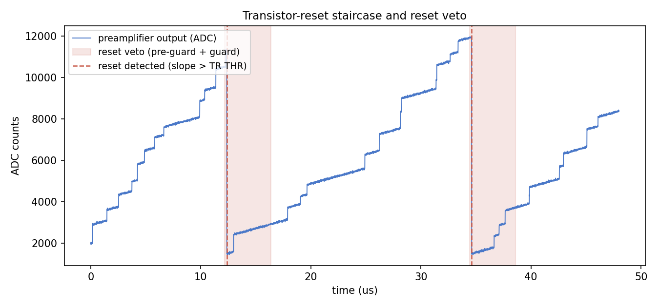
Building a multi-channel MCA for this kind of signal requires, besides the classic trapezoidal energy shaper, a set of dedicated features:

a reset detector that recognizes the reset edge and vetoes the trigger and the baseline restorer while the transient lasts;
a look-ahead (pre-guard) delay, so the veto also covers the samples immediately before the edge;
careful baseline management, because the input is a ramp and never flat;
pile-up rejection and rate/dead-time bookkeeping for quantitative spectroscopy.

This application note presents a complete, production-grade design for the x5560 family (DT5560 / R5560 / R5560SE, 125 MSPS, 14 bit): a 16-channel trapezoidal MCA implemented with Sci-Compiler, a full Python control GUI based on Sci-SDK and PyQt5, and the analysis tools (gaussian fit, Fe-55 energy calibration, dead-time corrected rates) needed to run a real spectroscopy measurement. The same firmware also works with SiPM / continuous-reset signals: with the reset threshold at its maximum the reset branch simply never fires and the design behaves as a standard trapezoidal MCA.

All the sources — the Sci-Compiler project, the generated firmware, the GUI and the documentation — are available in the repository linked at the bottom of this page.

To follow this application note you need Sci-Compiler 2026.4 or newer and SciSDK 1.2 or newer.

System architecture

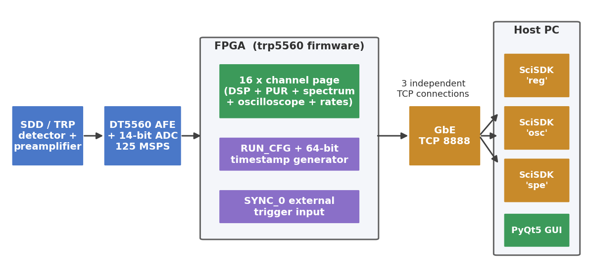
The FPGA hosts 16 identical channel pages built with the Sci-Compiler multichannel sub-design flow (see AN012 for the methodology): the sub-design is drawn once and instantiated 16 times, and every memory-mapped component inside it is automatically renamed page_chtrp_<N>_<name> in the generated RegisterFile.json. A single global register (RUN_CFG) acts as the run/configuration switch for all the channels, and a 64-bit timestamp generator is restarted on its rising edge.

On the host side the readout uses a feature of Sci-SDK that is worth highlighting: multiple AddNewDevice calls toward the same physical board, each with a different name, open independent TCP sockets. The GUI opens three of them:

sdk = SciSDK()
sdk.AddNewDevice("192.168.102.220", "DT5560", "RegisterFile.json", "reg")  # registers
sdk.AddNewDevice("192.168.102.220", "DT5560", "RegisterFile.json", "osc")  # oscilloscopes
sdk.AddNewDevice("192.168.102.220", "DT5560", "RegisterFile.json", "spe")  # spectra

so the (comparatively slow) waveform download never delays register access or spectrum polling, and each connection can be served by its own thread.

The channel processing chain

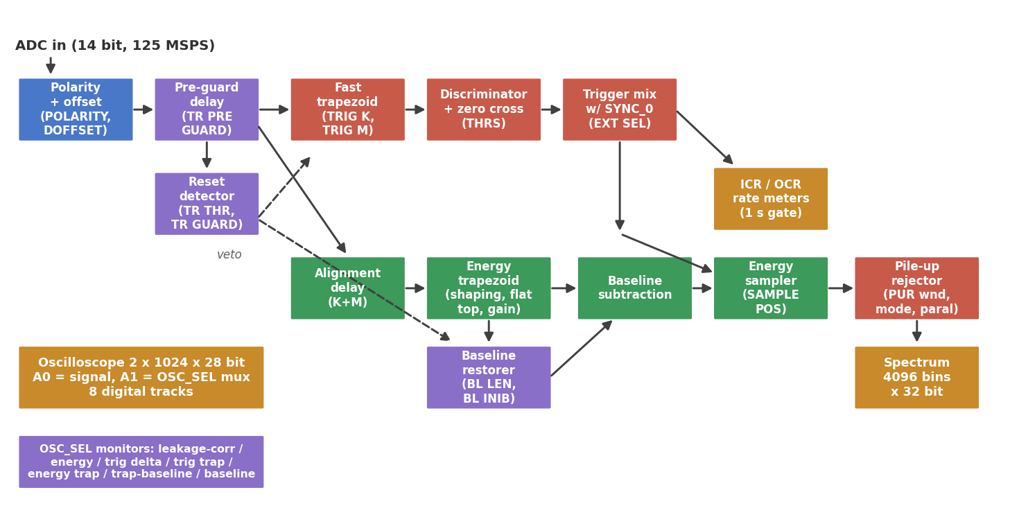
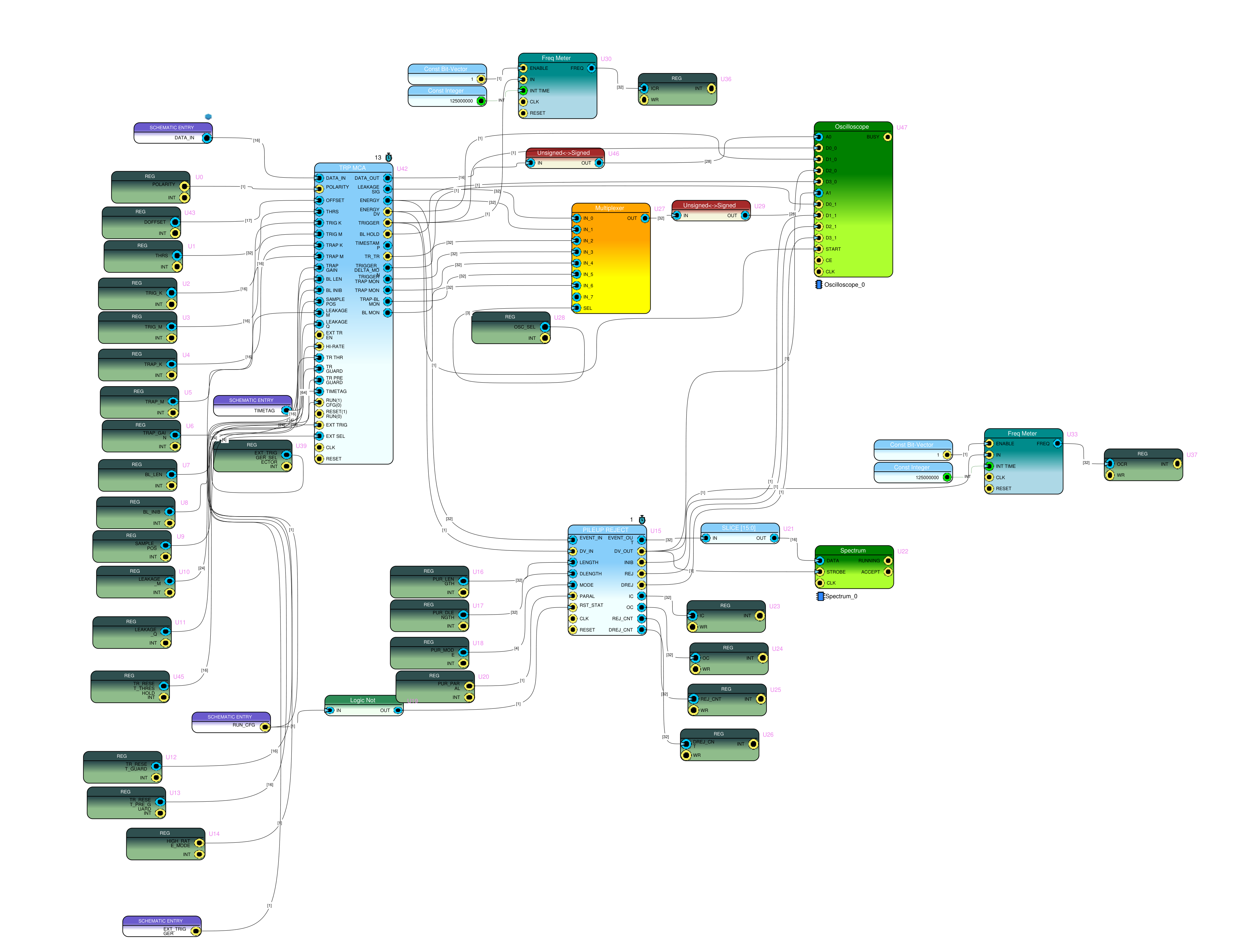
The heart of the channel is the TRP MCA block, a single HLS core that implements the whole pulse-processing chain at one sample per clock:

Polarity and offset — the 14-bit ADC stream is optionally inverted and shifted so that pulses are always positive steps.
Pre-guard delay — the stream entering the rest of the DSP is delayed by a programmable number of samples (the reset pre-guard). The reset detector watches the undelayed stream, so its veto reaches the shapers before the reset transient does.
Reset detector — a reset is declared when the signal drops by more than a programmable threshold within 4 samples (a slope discriminator, robust against the slow photon steps). The veto lasts a programmable guard time and, in normal mode, is extended by the baseline settling time; a high-rate mode skips the extension to minimize dead time per reset.
Fast trigger trapezoid — a short trapezoid (rise K, flat M, a few tens of ns) whose derivative is compared against the threshold; the trigger is validated on the zero crossing within 2·K samples, which gives a quasi-CFD behavior with very small time walk.
Trigger mixing with SYNC_0 — the internal trigger can be replaced by the external input, put in coincidence with it, or vetoed by it (internal, external, int AND ext, int AND NOT ext).
Energy trapezoid — the classic recursive Jordanov shaper. Its shape is defined by the shaping time (rise) and the flat top:

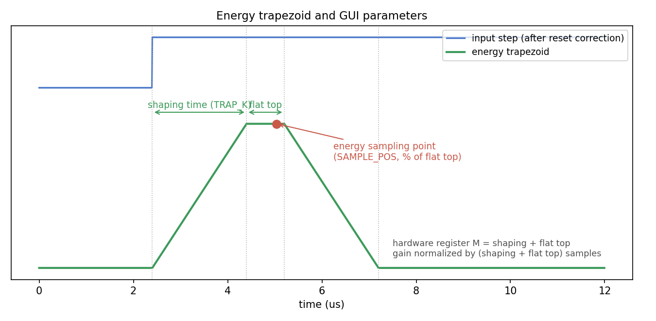
Trapezoid parameters

Two implementation details make the parameters detector-friendly:
- the hardware flat-top register actually holds shaping + flat top (the recursion uses the two delays K and M, with flat = M − K); the GUI does the conversion transparently;
- the digital gain is normalized by (shaping + flat top) in samples, so retuning the shaping time does not move the energy calibration.
Baseline restorer — a moving average (2^N samples) of the trapezoid, frozen for a programmable hold-off after every trigger and during the reset veto, subtracted from the trapezoid before sampling.
Energy sampler — samples trapezoid − baseline at a programmable position expressed as a percentage of the flat top (0% = beginning, 100% = end; out-of-range values are allowed for diagnostics).
Pile-up rejector — single-window or double-window (“peak-pair”: a second event inside the resolving window discards both events), paralyzable or non-paralyzable, with input/output/rejected counters.
Spectrum — a 4096-bin × 32-bit histogram with free-run, event-count or time-limited acquisition (millisecond resolution, live-time gated).
Rate meters — two frequency meters with a 1 s gate measure the trigger rate (ICR) and the accepted-event rate (OCR); their registers read directly in counts per second.
Oscilloscope — 2 analog traces × 1024 samples × 28 bit plus 8 digital tracks. Trace A0 is the conditioned input; trace A1 is selected at runtime by the OSC_SEL multiplexer among seven internal monitor points: leakage-corrected input, sampled energy, trigger delta, trigger trapezoid, energy trapezoid, trapezoid − baseline, and baseline. This turns every channel into its own debugging instrument: the trigger threshold, the flat-top sampling point and the baseline behavior can all be verified against the real internal signals.

The complete generated schematic of one channel page:

The control GUI

The repository ships a complete PyQt5 + pyqtgraph application (about 3000 lines) organized in four tabs, using the three-connection readout described above with one worker thread per connection.

Configuration

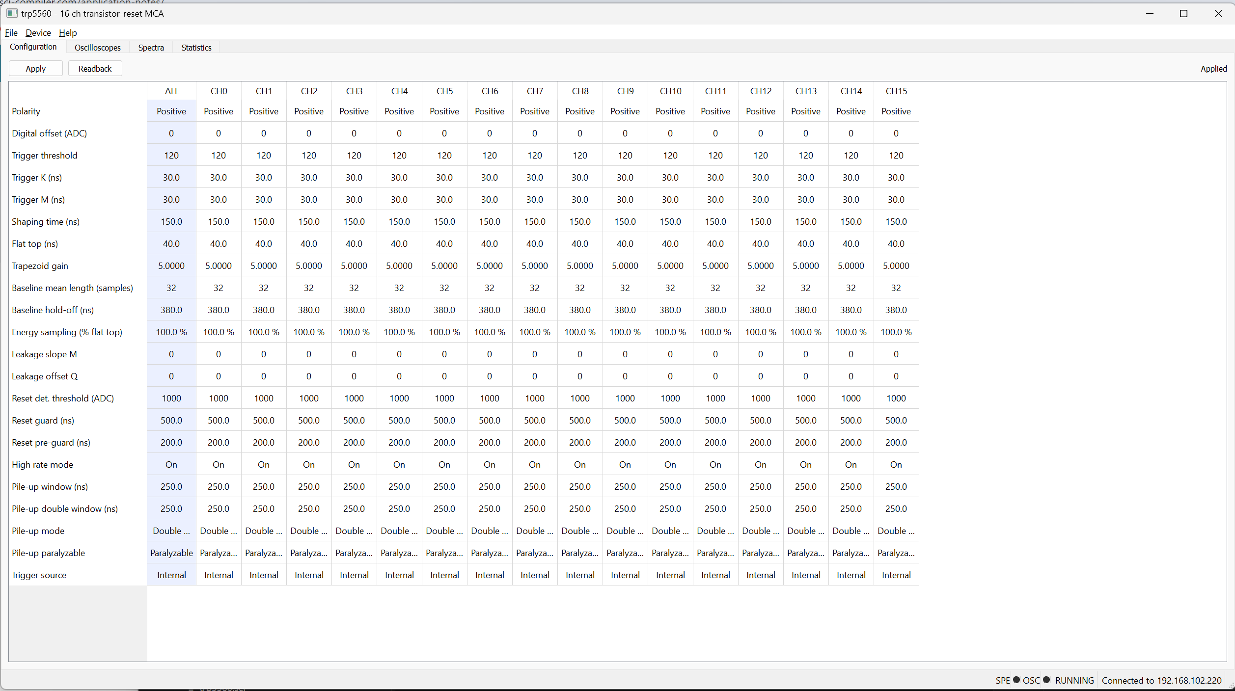
All the DSP parameters of the 16 channels in a single table: the ALL column propagates a value to every channel, time quantities are edited in nanoseconds and converted to 125 MHz samples, modified cells stay highlighted until Apply writes them. Apply performs the safe sequence RUN_CFG=0 → write → RUN_CFG=1 (the HLS parameters are declared ap_stable and must not change while running). Readback does the inverse conversion, including the derived quantities (flat top, sampling percentage, normalized gain). Cross-parameter constraints are enforced live — for example the baseline hold-off is never allowed below 2·shaping + 2·flat top.

Oscilloscopes

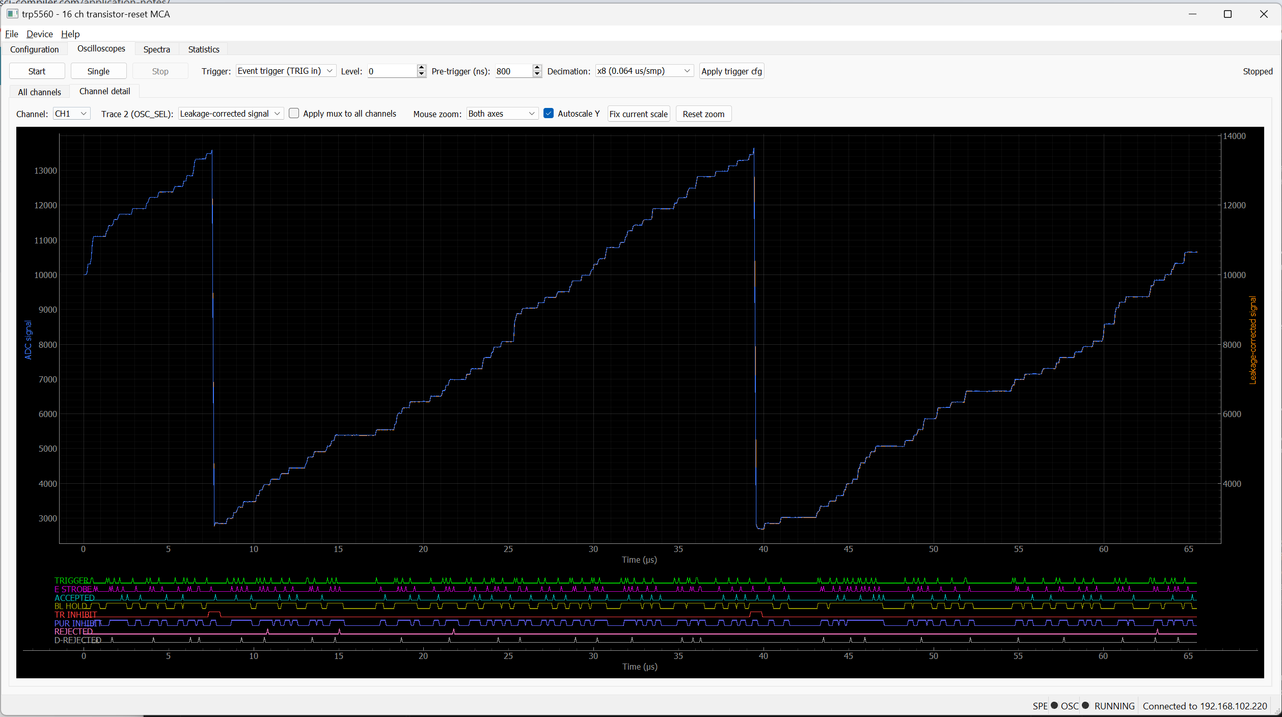
A 4×4 overview of the 16 scopes plus a detail view with the two analog traces on independent Y scales (the input staircase and the selected monitor have completely different ranges) and the 8 digital tracks rendered as a logic analyzer, X-linked to the analog plot. Continuous, Single (one waveform then stop) and per-axis zoom/autoscale modes are available. The event trigger of the scope is the channel’s own MCA trigger, so the displayed waveforms are exactly the pulses being measured.

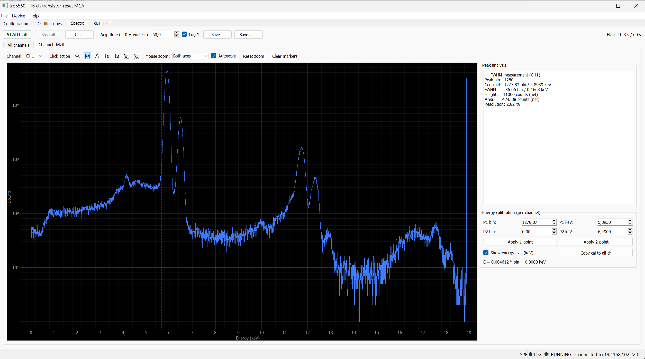
Spectra

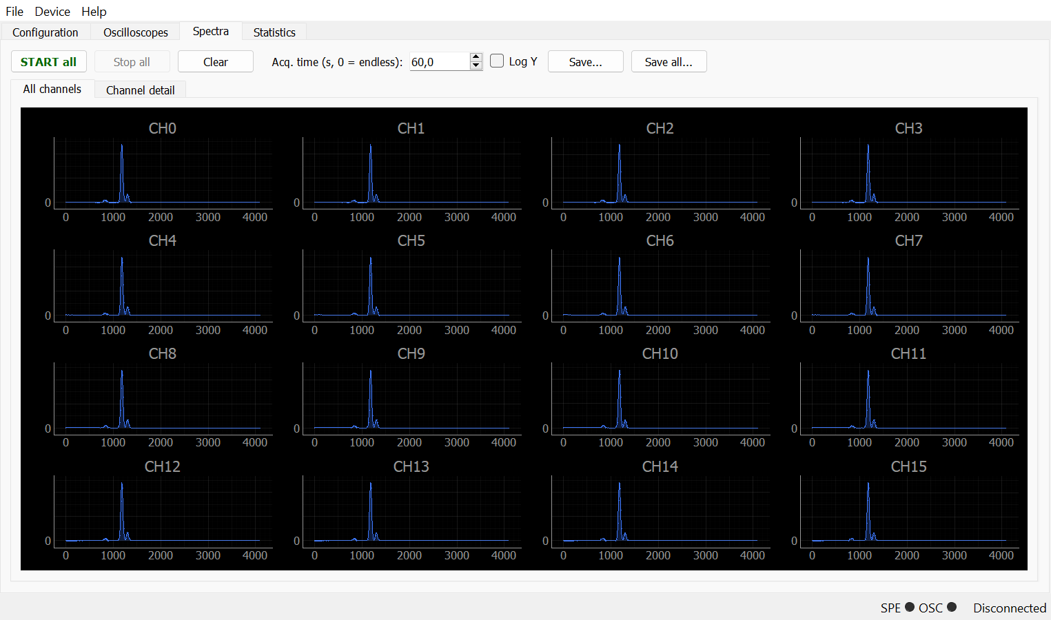
The 16 histograms with a synchronized START all (which also pulses RUN_CFG to restart the statistics and the timestamp from a clean state), programmable acquisition duration handled by the hardware time limit, logarithmic scale, and CSV / fixed-width TXT export. A click on any peak of the detail view can:

measure the FWHM numerically (interpolated half-maximum crossings);
run a gaussian + constant fit (centroid, sigma, FWHM, area, and resolution in % when calibrated);
set the calibration points;
run the Fe-55 quick calibration: one click on the Mn Ka peak performs the fit and calibrates at 5.895 keV; in the two-point variant the Kb peak is searched automatically at the position predicted by the Ka centroid, fitted with the Ka tail excluded from the window, and a two-point calibration (Ka + Kb at 6.490 keV) is applied.

Statistics and dead time

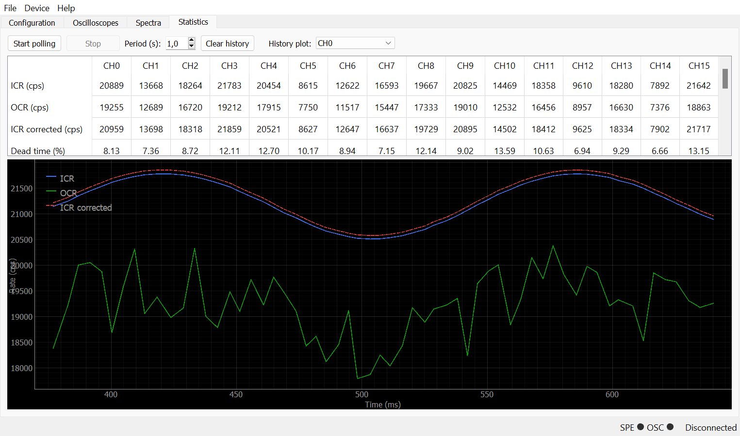
The statistics tab polls the per-channel counters (IC, OC, REJ, DREJ) and the 1 s gated ICR/OCR rate meters, and computes the dead-time corrected input rate. The dominant dead time of this architecture is the trigger trapezoid itself — two pulses closer than its width cannot be resolved — so each event blinds the discriminator for

tau = (2*TRIG_K + TRIG_M) * 8 ns

and the true input rate is recovered with the non-paralyzable model:

ICR_true = ICR / (1 - ICR * tau)
dead time % = 1 - OCR / ICR_true

A history chart tracks the rates of one channel (ICR, OCR, corrected ICR) or the ICR of all 16 channels over time.

Readout with Sci-SDK: the essential recipes

sdk.SetRegister("reg:/Registers/page_chtrp_3_TRAP_K", 250)      # 2 us shaping
res, icr = sdk.GetRegister("reg:/Registers/page_chtrp_3_ICR")   # cps, 1 s gate

Oscilloscope readout (non-blocking, so 16 scopes can be polled round-robin without stalling):

p = "osc:/MMCComponents/page_chtrp_0_Oscilloscope_0"
sdk.SetParameterString(p + ".data_processing", "decode")   # before AllocateBuffer
sdk.SetParameterString(p + ".acq_mode", "non-blocking")
sdk.SetParameterInteger(p + ".auto_arm", 1)
sdk.SetParameterString(p + ".trigger_mode", "ext")         # TRIG pin = MCA trigger
res, buf = sdk.AllocateBuffer(p)
res, buf = sdk.ReadData(p, buf)        # 0x300 = no waveform ready yet
# analog[s + 1024*ch], 28-bit two's complement in an int32;
# digital[s + 1024*track + 4096*ch], one byte per bit

Spectrum control with a hardware time limit:

p = "spe:/MMCComponents/page_chtrp_0_Spectrum_0"
sdk.SetParameterString(p + ".limitmode", "time_ms")
sdk.SetParameterInteger(p + ".limit", 60000)               # 60 s live time
sdk.ExecuteCommand(p + ".reset", "")                       # flush histogram
sdk.ExecuteCommand(p + ".start", "")
res, buf = sdk.ReadData(p, buf)                            # poll while running
counts = buf.data[0:buf.info.valid_bins]

Two practical notes that save debugging time:

enumerated parameters (trigger_mode, acq_mode, data_processing, limitmode) must be set with SetParameterString;
the oscilloscope decimator register is a linear reload counter: the decimation factor is value + 1 (any factor is legal, not only powers of two), and the pre-trigger register counts stored (post-decimation) samples.

Tuning procedure

A working bring-up sequence with an Fe-55 source:

Polarity / offset — free-run oscilloscope, check the staircase rises and stays inside the 14-bit range.
Reset detector — set the threshold above the steepest photon step; verify on the digital tracks that TR INHIBIT fires on every reset and on nothing else; adjust guard and pre-guard until the trapezoid shows no reset artifacts.
Trigger — watch the Trigger delta monitor, set the threshold just above the noise band; verify the TRIGGER digital track.
Energy shaping — choose the shaping time from the noise corner of the detector (1–4 µs typical for SDD), a flat top longer than the ballistic deficit, and place the sampling point with the Trapezoid − baseline monitor (default 80% of the flat top).
Gain — set the normalized gain so the Ka peak falls in the upper half of the 4096-channel range without exceeding it.
Calibrate — acquire a spectrum, one click on the Ka peak with the Fe-55 Ka+Kb quick calibration.
Rates — enable statistics polling and verify the dead-time figures while adjusting the pile-up windows.

Source code

The complete project — Sci-Compiler design, generated firmware for DT5560, Python GUI, self-tests and documentation (user guide with all the parameter semantics, plus an AGENT/ knowledge base with the firmware and SDK internals) — is available in the repository below.