Case-Study Case-Study, Detector, Spectroscopy, Monitoring
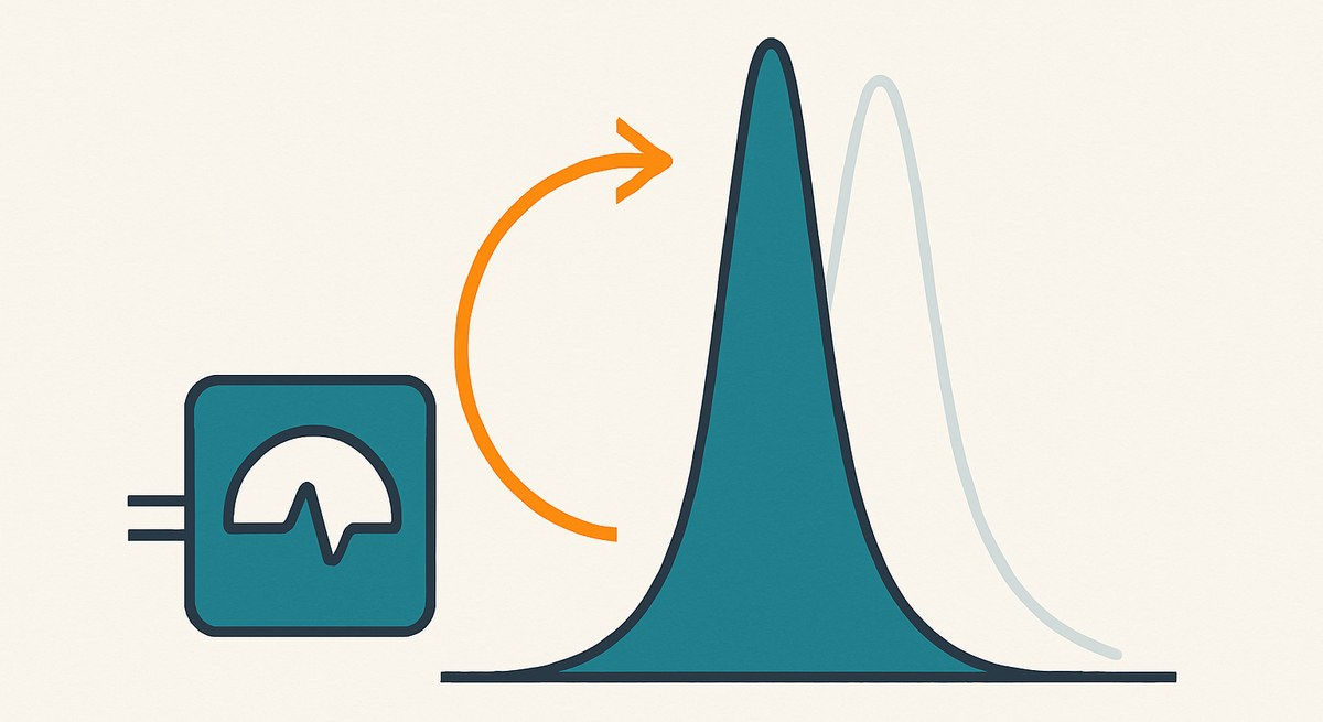
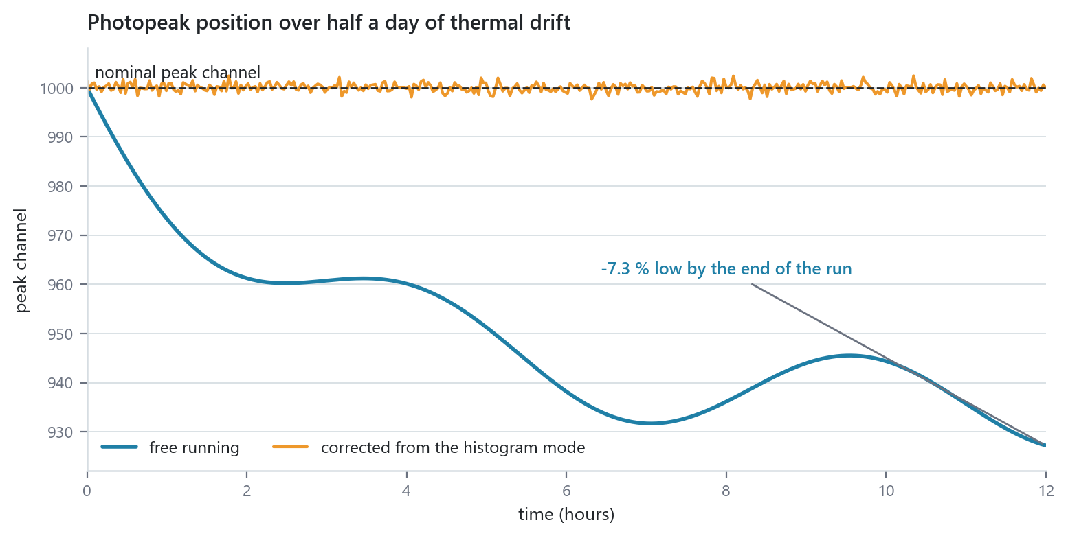
A silicon photomultiplier changes its gain by roughly one percent per degree. A photomultiplier tube drifts with supply, with count rate and with its own history. Over a long acquisition, both smear the photopeak, and the resolution you quote is not the resolution the detector has, it is the resolution the detector had averaged over the drift.
The usual fix is to put the correction in software: read out spectra periodically, fit the peak on the host, compute a correction, write it back. This works, and it has three properties nobody likes. The loop is as slow as the readout and the fit. The correction depends on a PC being alive and running the right program. And the raw data on disk is uncorrected, so every reprocessing has to redo the same work.
Doing the measurement in the device
The Histogram Analyzer block changes what is possible here, because it does not just accumulate a histogram, it also analyses one.
The binner takes one sample per clock. Alongside it, and independently, a scanner walks the histogram and extracts: total, lowest and highest occupied bin, range, mode and mode count, median, four configurable quantiles, IQR, mean, variance, standard deviation, skewness, kurtosis, four configurable threshold occupancies, FWHM, FWTM, and a sub-bin peak position by parabolic interpolation.
That list is the reason the loop can close in hardware. The peak position is not something you have to fit on a host; it is a pin. Every statistic can be switched off, which removes both its output and its logic before synthesis, so a design that only needs the peak position pays only for the peak position.

The loop is then trivial: compare the reported peak position against the nominal channel and drive the bias or the digital gain trim to null the difference. It runs at whatever rate the scan completes, needs no host, and keeps running when the DAQ PC is rebooted.
Integrity outputs, which are not optional
The Histogram Analyzer emits a set of outputs that exist because without them every number above can be silently wrong: BIN_SATURATED, SAT_BINS, UNDERFLOW, OVERFLOW, NONEMPTY_BINS and LOST.
This matters more in a control loop than in a display. A histogram whose bins have saturated still has a mode, and that mode is meaningless; a loop that acts on it will drive the detector somewhere bad with complete confidence. Gating the correction on the integrity flags is what makes the difference between a stabiliser and a fault amplifier.
Input conditioning is fully runtime: subtract a BASE, rebin by a SHIFT, clamp to MAX_BIN. So the analysed window can be zoomed onto the photopeak without re-synthesising, which is what you want, since a mode computed over a window containing only the peak is far better conditioned than one computed over the whole spectrum.
Choosing the mode
Three operating modes trade dead time, memory and snapshot consistency against each other, and the choice is a real one.
FREEZE stops binning while the scan runs. The snapshot is perfectly consistent and you pay dead time.
DOUBLE ping-pongs between two buffers: no dead time, consistent snapshots, twice the memory.
LIVE never stops and uses a single buffer. It needs gaps in the input stream, and it is worth understanding why, because the reason is also the reason it works. A BRAM read is synchronous, so a sample accepted on clock c is only visible to a read issued two clocks later. The gaps are what give the scanner its access to the memory, and that same rule is what makes clear-on-scan race free rather than merely usually fine. For a spectroscopy chain, where events are sparse compared to the clock, the gaps are free.
What else the loop can watch
Since the statistics are there, the loop can be made to notice more than drift.
The FWHM output is a resolution monitor: a photopeak that widens without moving is not a gain problem, it is noise or a failing detector, and a stabiliser that silently corrects gain will hide that. Watching both is what separates the two failure modes.
Skewness of the peak region detects the low-energy tail that develops from charge collection problems or from pile-up at rising rate. Mode count against total is a live measure of peak-to-background.
None of these need the host either.
This is a reference design. The block behaviour and the output list are as documented; the drift figure is computed from a thermal-drift model, not measured on a detector.