Case-Study Case-Study, Multi Channels, Detector, Monitoring
A 16-channel SiPM array, a multi-anode PMT, a strip detector, a segmented drift chamber. They all share a problem that a single-channel instrument does not have: at any moment, some channel is probably misbehaving, and nobody knows which.
A dead channel produces a flat baseline and no events. A noisy channel produces a rising trigger rate and pollutes coincidences. A channel with a drifting baseline slowly walks out of its threshold. On a two-channel detector, you notice. On a 64-channel one, you notice weeks later, in the analysis, and you throw away the data.
What is needed is not clever. It is a handful of simple numbers per channel, continuously, without a host and without occupying the readout bandwidth.
The numbers worth having
The Statistics plugin has twenty-five per-operator block statistics, each computing one quantity over a runtime-sized block of N = 2^EXP samples. Four of them answer nearly the whole question.
Block Mean is the baseline. Its drift over hours is the slow-control quantity that predicts a channel walking out of threshold before it does.
Block Slope Stats gives the standard deviation of the first difference. This is the better noise estimator on a real detector, and the reason is worth stating: because the first difference deletes any constant offset, its sigma does not see slow wander at all. Block Std Dev on a drifting channel reports the drift as if it were noise. Slope sigma reports only the sample-to-sample roughness, which is what “noise” was supposed to mean. For white noise of standard deviation s it converges to s·√2.
Block Zero Crossings counts how often the signal crosses a runtime LEVEL. It is the cheapest frequency estimator that exists, one comparator and one counter, and on a detector channel it is a discriminator-free event-rate monitor: put a slow baseline tracker on the LEVEL pin and the crossing count is the activity of that channel.
Block SNR is mean over sigma, taken as a linear ratio. On a DC-ish measurement corrupted by additive noise, which is exactly what a detector baseline is, it is the natural figure of merit.
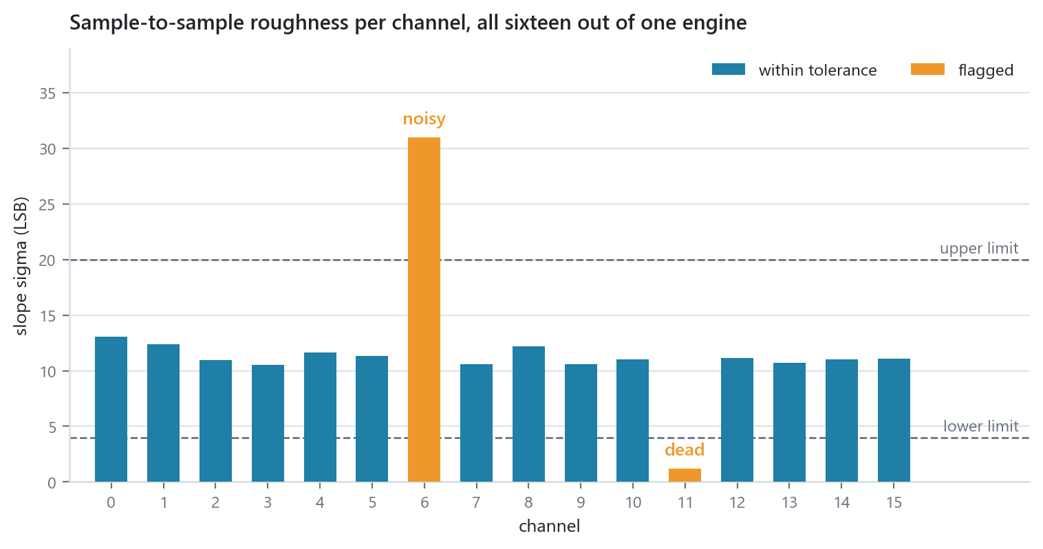
Two channels fall outside the band and both failure modes are visible at once: one channel is roughly three times noisier than its neighbours, and one is essentially flat, which on a detector that should be seeing something is not a good sign.
Why this is affordable
The obvious objection is that sixteen channels means sixteen copies of every statistic, and a divider or a square root is not free.

Every one of the twenty-five statistics has a time-multiplexed twin. The contract is worth understanding because it explains where the saving comes from — and if the packing convention is new to you, what a TM signal is covers it properly.
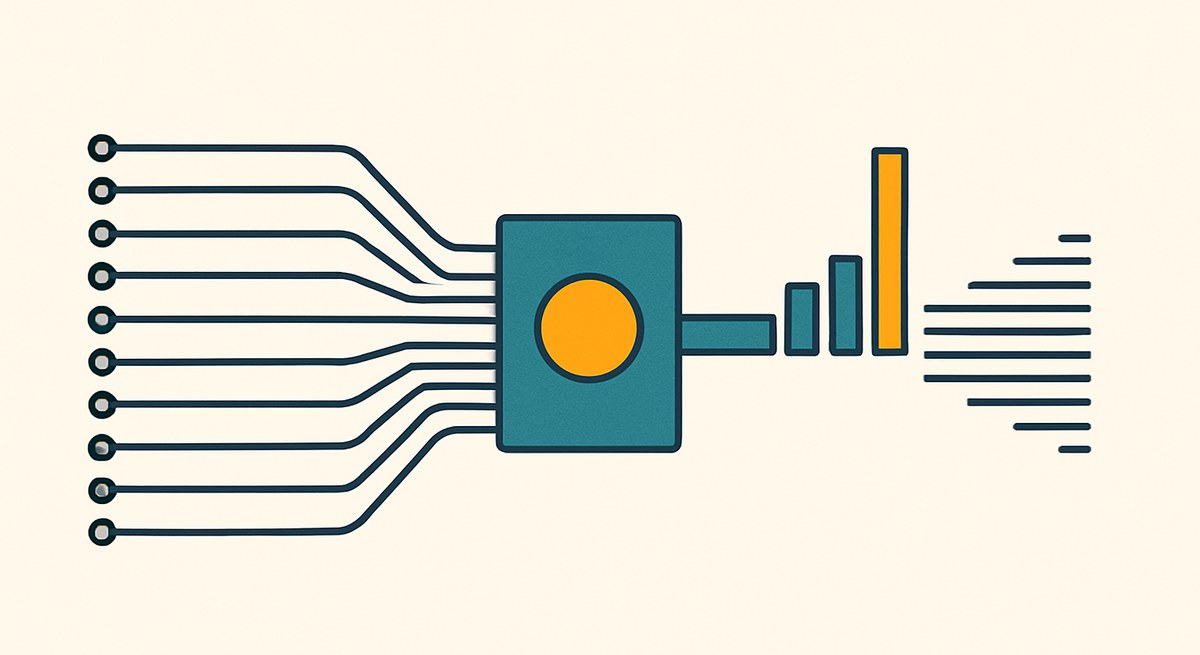
The channels get onto the shared bus through the TM Packer, which concatenates N independent scalar signals into one TM word, and come off it through the TM Splitter or the TM Phase Extractor. Between 2 and 16 independent channels are packed on one wide bus, lane 0 in the low bits, sharing one frame: one runtime EXP pin, one IN_DV, one OUT_DV, scalar BUSY and SAMPLE_COUNT. The accumulators and the per-lane state are strictly per lane — they have to be, since sharing any of them would bleed one channel’s history into another. But there is one serial engine set serving the lanes one after another, so the dividers, the square roots and the wide once-per-block products stay single no matter how many lanes there are.
That asymmetry is the whole economics. Accumulators are registers and adders, and sixteen of them are cheap. Dividers and square roots are not, and there is one.
The cost is time rather than area: the lane-multiplexed tail is L_tm = TM·(L_scalar − 1) + 1. For a diagnostic computed once per block over thousands of samples, that is invisible.
What to do with it
The output is a small, slow, fixed-size record per channel per block. It costs almost nothing to read out next to the event data, and it is the same record whether the detector has 4 channels or 64.
From there the useful things are the boring ones. Threshold it and raise an alarm. Log it and plot the history, so that a channel that has been slowly degrading for a month is visible as a trend rather than as a surprise. Feed it to the trigger, so that a channel currently outside tolerance is automatically excluded from coincidences instead of poisoning them. Gate the run start on all channels being in band, so a run does not begin with a dead channel nobody checked.
The general point
An array detector without per-channel diagnostics is not sixteen detectors, it is one detector with sixteen ways to fail quietly. The block statistics make the monitoring cheap enough that there is no longer a reason to leave it out, and the time-multiplexed twins make it cost roughly the same at sixteen channels as at one.
This is a reference design. The block behaviour, the TM packing contract and the latency formula are as documented; the per-channel figure is illustrative data, not measured on a detector.