Case-Study Case-Study, DSP, Signal Processing, Trigger
If you know the shape of the pulse you are looking for, the filter that maximises the signal-to-noise ratio at the moment of detection is the matched filter: correlate the incoming stream with a time-reversed copy of that shape. This is not a heuristic, it is the optimum, and for a detector pulse buried in white noise nothing else does better.
The reason it is not used everywhere is arithmetic. A matched filter is a FIR whose length is the length of the pulse. A scintillator pulse sampled at 125 MS/s is easily several hundred samples long. A 512-tap FIR at the full sample rate is 512 physical multipliers running at 125 MHz, which on most devices is the entire DSP budget spent on one channel of one filter.
So the usual compromises appear: shorten the filter and accept a worse SNR, run it on a decimated stream and accept worse timing, or replace it with a trapezoidal shaper, which is the matched filter for a step, not for your pulse.

Doing it in the frequency domain
Convolution in time is multiplication in frequency. The FFT Filter block exploits that directly: it transforms a block of input, multiplies bin by bin against the stored spectrum H[k] of the filter, and transforms back. Overlap-save at 50 % stitches the blocks together so that the output is a continuous stream with no seams.
The cost of this is two pipelined FFT cores and one complex multiplier, and it does not grow with the length of the impulse response. A filter of N/2 taps costs the same as a filter of 8 taps. That is the entire argument: past a few tens of taps, fast convolution is cheaper, and by the time you reach the hundreds of taps a matched filter actually needs, it is not close.
The block runs at the full input rate. This is worth emphasising because FFT-based filtering is often assumed to require gaps in the input; here the two cores ping-pong so that one transforms while the other loads.
What it buys
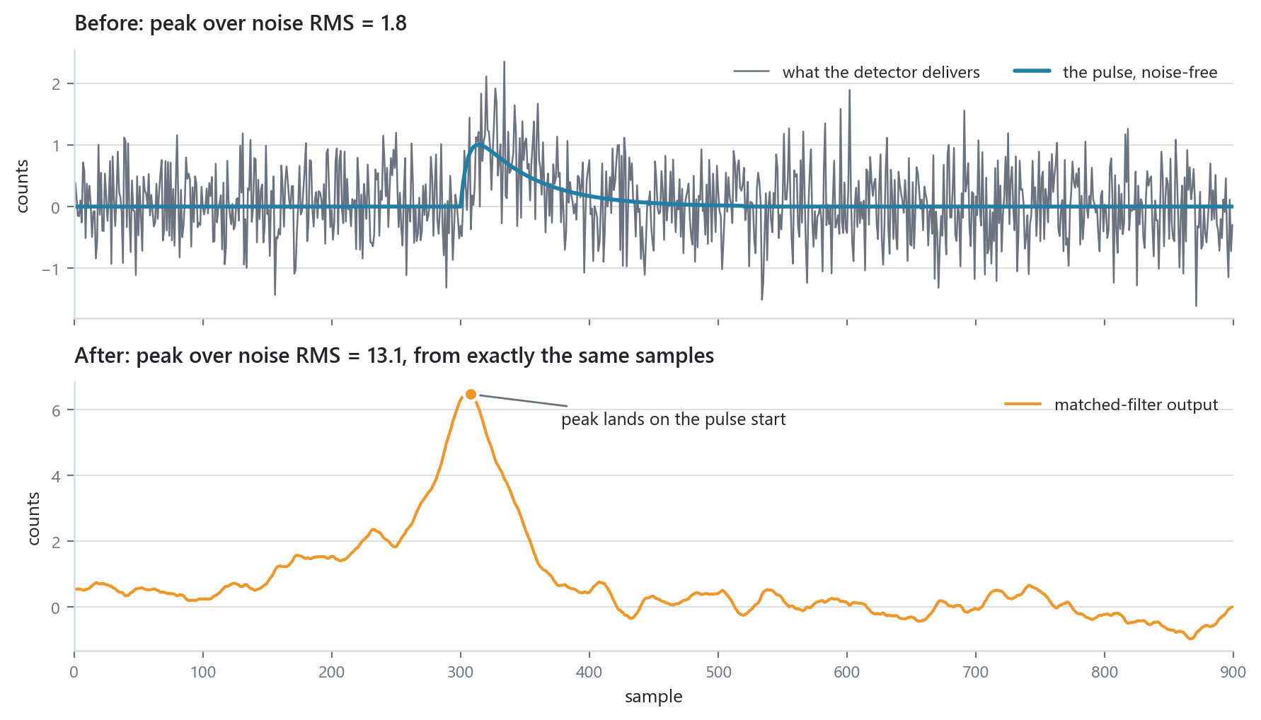
Same samples, same noise, one block in between. The peak-to-noise ratio goes from under 2, where a threshold trigger would be firing on noise as often as on pulses, to over 13, where it is not.
The peak of the output lands on the start of the pulse, which makes the output directly usable as a trigger: threshold the filtered stream instead of the raw one and both the efficiency and the false-trigger rate improve at once.
Where H[k] comes from
The filter is only matched if the template is actually your pulse shape. There are three ways to get it, in increasing order of honesty.
Draw it. The FFT Filter designer lets you specify the response from presets or by dragging editable points, or load coefficients from a file. This is fine when you know the shape analytically.
Measure it, which is better. The Waveform Averager block exists for exactly this: it coherently averages a programmable power-of-two number of triggered waveforms and its pile-up aware mode discards any waveform contaminated by a second trigger, so what accumulates is a clean template rather than a mixture. Average a few thousand real pulses from your detector and you have the true shape, including whatever your preamplifier did to it.
Load it at runtime, which is better still. FFT Filter Prog is the same engine with H[k] held in RAM and written over COEF_ADDR / COEF_DATA. The template becomes a parameter of the run rather than of the bitstream, which means it can be re-measured after a temperature change, adapted per channel, or swapped when the detector is changed, all without re-synthesising.
That last combination, Waveform Averager building a template that FFT Filter Prog then loads, closes a loop that is normally done offline on a PC, entirely inside the device.
The price
Fast convolution has one cost that a direct FIR does not: latency. The block has to fill before it can transform, so the output lags the input by of order the transform length. For pulse detection and spectroscopy this is irrelevant, since a few microseconds of fixed, known delay changes nothing. For a fast veto or a coincidence window it may not be, and there the honest answer is a short direct FIR and a worse SNR.
The other thing to keep in sight is that a matched filter is matched to one shape. If your detector produces two populations with genuinely different shapes, the filter is optimal for one and merely good for the other, and telling them apart is a different problem with a different answer.
This is a reference design. The block behaviour is as documented; the figures are computed from a simulated detector pulse in white noise, not measured on an instrument.