Case-Study Case-Study, DSP, Signal Processing, Detector
Whenever a measurement can be repeated on demand, averaging is the cheapest signal-to-noise ratio available. Pump-probe spectroscopy, time-of-flight measurement, LIDAR return profiling, ultrasound, laser-induced breakdown, and the routine business of extracting a detector’s pulse shape all share the same structure: fire something, capture the response, do it again.
The noise is uncorrelated between shots and the signal is not, so averaging N waveforms improves the amplitude signal-to-noise by √N.
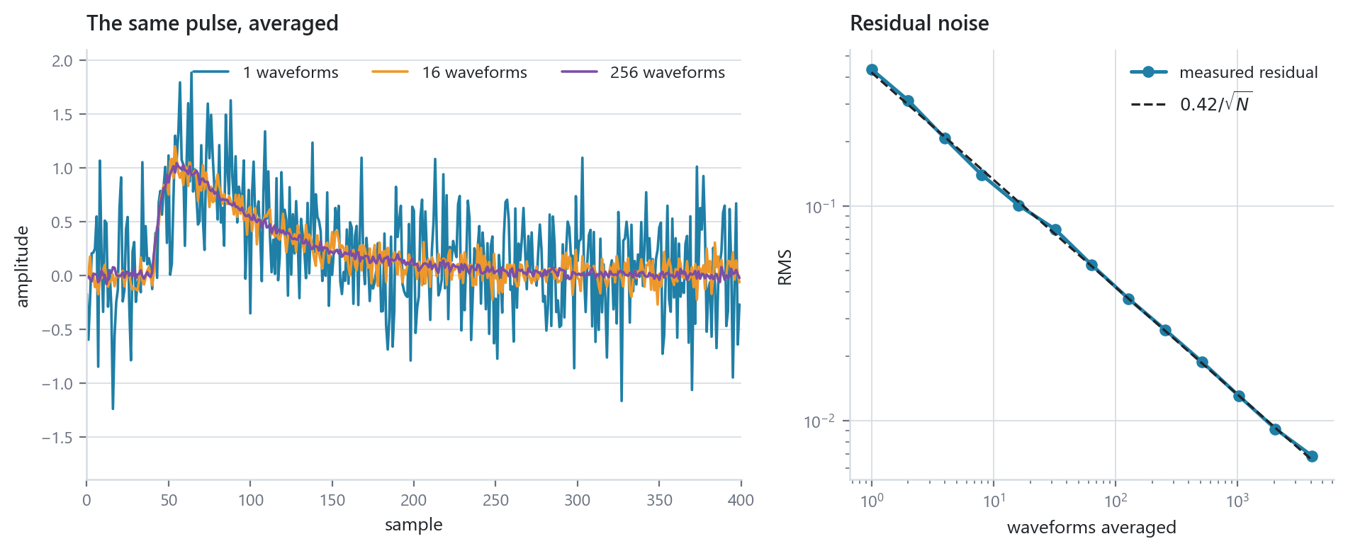
The right panel is worth a moment. The measured residual follows σ/√N over four decades with no departure, which is what tells you the averaging is genuinely coherent — that the waveforms really are being aligned to the same time origin. Any trigger jitter, any timebase drift, and the curve would flatten out at the level set by the misalignment. A √N plot is therefore not just an illustration, it is the diagnostic for whether your averaging is working.

Two design decisions worth knowing about
The Waveform Averager sums a programmable power-of-two number of waveforms, sample by sample, into a 36-bit accumulator RAM, and streams the result out as a burst. Both the number of averages and the waveform length are runtime inputs.
Two things about it are not accidental.
The output emits at power-of-two totals, and the block contains no divider at all. Dividing by an arbitrary N would mean a divider in the datapath; restricting N to powers of two makes the division an arithmetic shift, which is free. The number of averages is still a runtime choice, it is just a choice from the powers of two, which for this application costs nothing — nobody needs to average exactly 1000 waveforms rather than 1024.
The history can be cleared after each output or kept indefinitely. Clear-and-restart gives independent successive averages, which is what you want when the thing being measured is changing. Cumulative keeps improving the same estimate, which is what you want when it is not.
The pile-up guard
The feature that distinguishes this from a summing loop anyone could write is the pile-up aware acquisition mode: any waveform contaminated by a second trigger inside the acquisition window is discarded entirely.
This matters because pile-up does not average out. Random noise is symmetric and cancels; a second pulse landing somewhere in the window is always additive, and it always lands at a random position, so what it contributes to the average is a broad positive pedestal that grows with rate. A template built from a piled-up sample is not a noisy template, it is a wrong one, and it is wrong in a way that gets worse exactly when the experiment gets interesting.
Throwing the whole waveform away costs statistics and buys correctness, and given that averaging is cheap, that is the right trade.
Note that the START input is deliberately level sensitive for triggering but edge sensitive for pile-up detection. That asymmetry is what lets the block handle back-to-back triggers correctly rather than mistaking a legitimately adjacent waveform for contamination.
Where the template goes
For the pulse-shape case, the averaged waveform is not the end product, it is a parameter for something else.
A clean template is what a matched filter needs. Average a few thousand real pulses, take the conjugate of its spectrum, and load that into FFT Filter Prog over its runtime coefficient bus. The result is a matched filter tuned to the detector you actually have, in the state it is actually in, rather than to an analytic pulse shape from a textbook.
Because both halves run in the device, this can be repeated: re-measure the template after a temperature change or a bias adjustment and reload it, without re-synthesising and without a host in the loop.
Scaling and limits
There is a Waveform Averager TM twin, so an array detector can average every channel through one engine.
The limit to be aware of is the one every coherent average has: it assumes the signal is identical shot to shot and only the noise differs. If the real quantity varies between shots — an amplitude that fluctuates, a time-of-arrival that walks — the average smears it and you have measured something that never happened. When the variation is the measurement, averaging is the wrong tool and a per-shot statistic is the right one.
This is a reference design. The block behaviour is as documented; the figures are computed from a simulated pulse in white noise, not measured on an instrument.