Case-Study Case-Study, DSP, Signal Processing, Monitoring
Some of the most useful measurements an instrument makes are not of the thing it was built to measure. A cryostat develops microphonics from a pump that was fine last month. A detector picks up a switching supply through a ground loop. A beam becomes unstable at a frequency that tells you which magnet is at fault. A mechanical stage starts to resonate.
All of these appear as a narrow line in the spectrum of a signal you are already digitising. The question is whether your instrument is in a position to notice.

The two decisions
A continuous spectral monitor is a short chain, and essentially all of its behaviour is set by two choices.
Which window
This is the decision people get wrong, usually by not making it. A finite block of samples is an infinite signal multiplied by a rectangle, and that multiplication smears every tone across the whole spectrum. The window is what you replace the rectangle with, and every window is a different bargain between two things you cannot have at once.
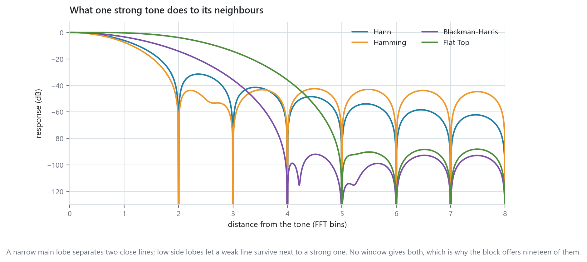
Read this figure as: a single pure tone sits at bin 0, and the curve is what it does to every other bin. The Hann window has a narrow main lobe, so two tones two bins apart stay distinguishable, but its side lobes are only about 30 dB down near the peak, so a line 40 dB weaker than a nearby strong one is buried. Blackman-Harris pushes the side lobes below 90 dB, and pays for it with a main lobe twice as wide. Flat Top is wider still, and is not there for resolution at all: it is the window you use when the number you want is the amplitude of a line, because it makes the response nearly flat across a bin so the answer barely depends on where the tone fell.
There is no window that is best. Which is why the FFT Windowed block offers nineteen families, designed in a graphical designer with a test-tone simulator so you can see what a given choice does before committing it. The question the designer really answers is: given what I am hunting for, which of these bargains do I want?
How much averaging
The second decision is what to do about variance. A single 1024-point spectrum of a noisy signal has enormous scatter, bin to bin, and that scatter is what hides a weak line.
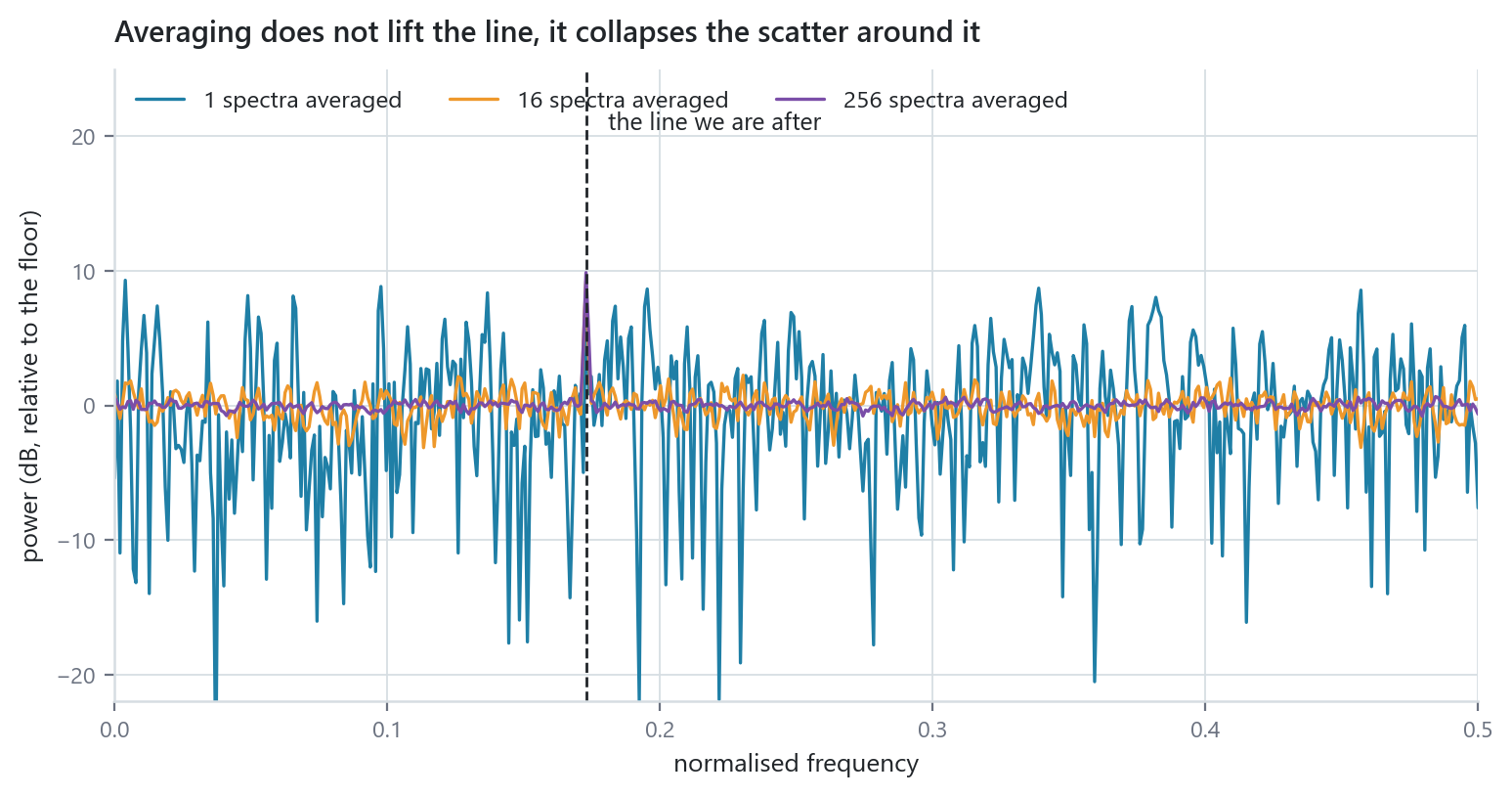
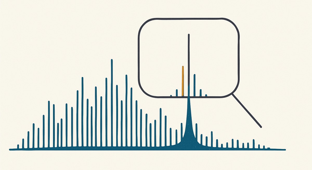
The important thing about this figure is what does not happen. Averaging does not raise the line: it sits the same number of decibels above the noise floor in all three traces, because averaging power spectra reduces the variance of the estimate, not the noise itself. What changes is that the floor becomes a floor instead of a thicket. With one spectrum the line is indistinguishable from a dozen noise peaks of the same height. With 256 it is the only thing standing.
The FFT Average block does this bin by bin over a programmable power-of-two number of spectra, with the count as a runtime input. It is double buffered, so no input spectrum is dropped while a result streams out.
Reading it back
The averaged spectrum feeds the Spectrum readout block and lands in the Resource Explorer, which added the things you need for this specifically: a statistics side panel with region-of-interest support, so you can put a box around the suspect line and get its area and peak directly, and a log-Z toggle, without which a spectrum with 60 dB of dynamic range is a flat line with one spike.
The shape of the design
What makes this practical is that it is permanently on. The chain is a handful of blocks sitting behind an ADC that is already there, using an FFT core the design may already contain, and it costs no host bandwidth because only the averaged spectrum is read out, at whatever rate you choose to look at it.
That is the difference between spectral analysis as a diagnostic activity, where somebody notices a problem, connects an analyser and hunts, and spectral analysis as a permanent instrument function, where the line was in the log at the moment it appeared.
For multi-channel instruments, both the windowed FFT and the averager have time-multiplexed twins, so the same monitor can cover every channel with one engine.
This is a reference design. The block behaviour is as documented; the window responses are computed from the standard window definitions and the averaging figure from simulated data, not measured on an instrument.