Case-Study Case-Study, Signal Generation, Testing, Detector
Testing a spectroscopy chain properly requires a detector, a source, a licence to hold the source, a room to hold it in, and hours of acquisition to get the statistics. Which is why, in practice, firmware changes are usually tested against a pulse generator producing identical pulses at a fixed rate.
That test proves the chain can process a pulse. It proves almost nothing about the things that actually break: pile-up handling at realistic rates, dead-time accounting, baseline restoration under a varying load, the energy resolution the filter really delivers, or whether the spectrum that comes out has the right shape.
The gap between the two is where bugs live, and it is a gap that can be closed entirely inside the device.

Building a detector out of three blocks
Poisson Pulser. On every clock a Bernoulli trial fires a one-clock pulse with probability RATE/2^32. That gives genuine Poisson arrival statistics with geometric inter-arrival times, which is what a radioactive source produces and what a function generator emphatically does not. Pile-up therefore appears on its own, at the right rate, with the right distribution, without anyone arranging it. RATE is a 32-bit runtime pin, so it can be driven from a register and swept during a test.
Random Generator (Arbitrary Distribution). This is the block that makes the exercise meaningful. It produces random values whose histogram reproduces any distribution you give it, using inverse transform sampling: tabulate the CDF, draw a uniform number, binary-search for the bin it falls in, and that bin index is the sample. Because the CDF is monotonic the search is a binary search, which is why the block costs one table and one comparator, with no multiplier and no divider anywhere.
The distribution is chosen in a Distribution Designer, and it ships with 58 real measured isotope spectra alongside 20 analytic shapes and file import. So the amplitudes you inject are not Gaussian-around-a-value, they are the shape of an actual source, with its Compton continuum and its escape peaks and its background.
Coloured noise. A real baseline is not white. The plugin has pink noise at −3 dB/octave by the Voss-McCartney method, brown at −6 dB/octave from a leaky integrator, plus exponential and Rayleigh sources. Adding 1/f is what makes a baseline restorer face the problem it was written for.
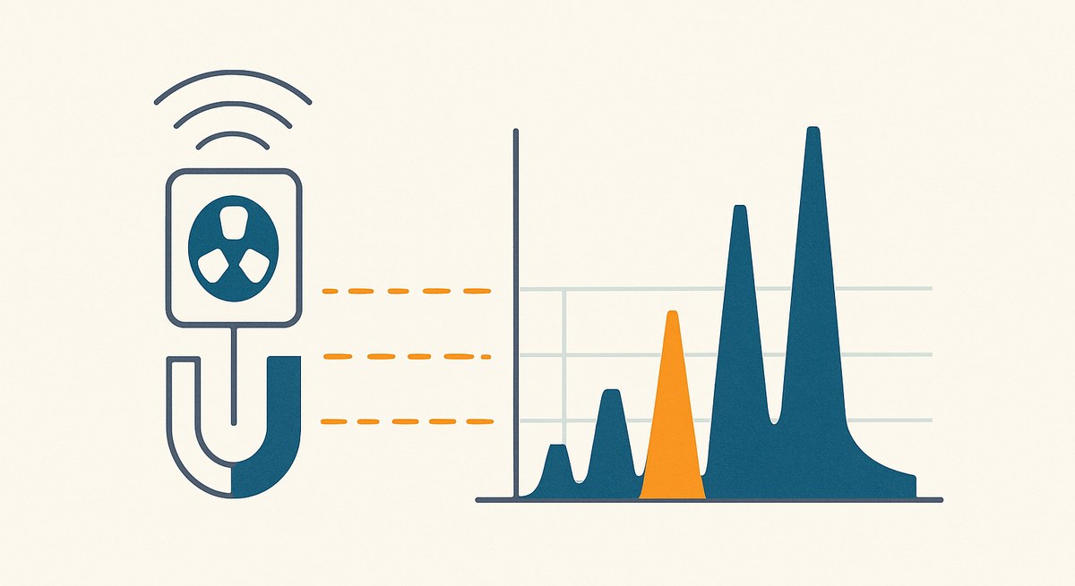
These three feed a shaper that turns each amplitude into a pulse of the right shape, and the result goes into the real chain: the real energy filter, the real trigger, the real histogram, the real readout.
The test that this makes possible
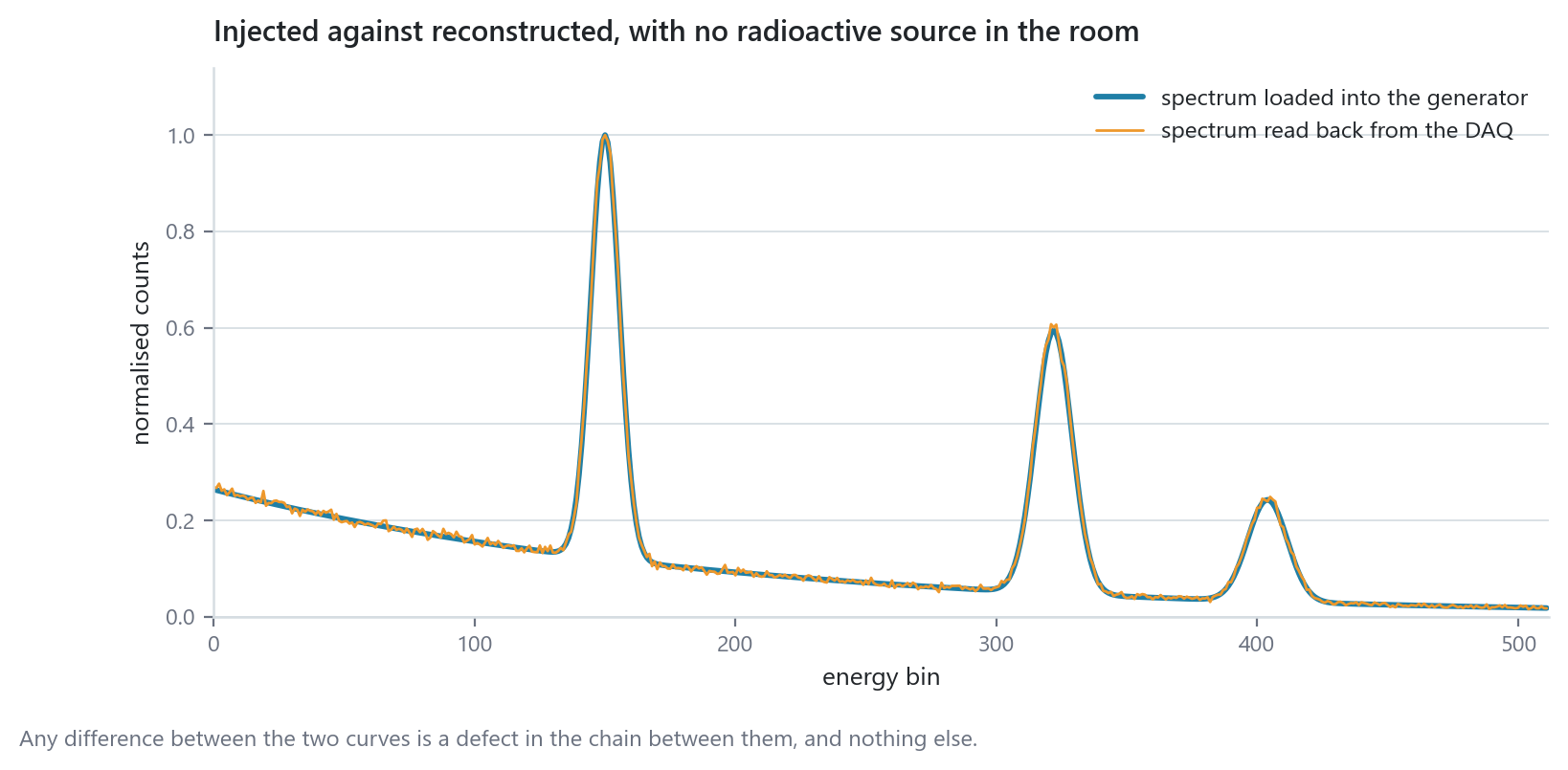
The measurement is now a comparison between two things you have both of: the spectrum you loaded into the generator, and the spectrum the chain reconstructed. Any difference between them is a defect in the chain between them, and nothing else. There is no detector physics in the way, no source strength to correct for, no geometry.
That is a qualitatively different kind of test from “the peak is roughly where we expected”.
Some specific things it catches:
Resolution the filter really delivers. Inject a delta-function line and measure the FWHM out. The difference is the filter’s own contribution, with no detector broadening mixed in.
Pile-up and dead time. Sweep RATE across two decades and watch the reconstructed spectrum degrade. The rate at which the peak starts to shift or the throughput turns over is a number about your firmware, measured directly.
Baseline restoration. Turn the pink and brown noise up and down and see how far the peak moves.
Linearity. A spectrum with lines at known positions gives you the integral non-linearity of the whole chain in one acquisition.
Where this pays off most
The generator is deterministic when you want it to be. The seeds are auto-randomised per instance so that multiple blocks are independent, but they stay editable, and RESET restarts the sequence identically. So a test can be exactly repeatable, which is what turns it from a demonstration into a regression test.
Combined with the Docker image for CI/CD pipelines, this means a firmware change can be validated against a full synthetic acquisition automatically, on every commit, with the pass criterion being a comparison against the injected spectrum. No hardware in the loop, no source, no operator.
The other place it pays is early. The DAQ software, the readout, the histogramming and the analysis can all be developed and debugged against a design that produces realistic data, months before the detector exists.
What it does not replace
An emulator tests the chain from the ADC onwards. It says nothing about the analog front end, the preamplifier noise, the actual detector response, or the cabling — all of which are also capable of ruining a measurement.
The right way to think about it: it removes the firmware from the list of suspects, so that when you finally connect the real detector and something is wrong, you know where it is not.
This is a reference design. The block behaviour, the sampling method and the shipped spectrum library are as documented; the spectra shown are computed from a synthetic source model, not measured on a detector.