Case-Study Case-Study, Signal Generation, Testing, DSP
“Add some noise and see if it still works” is one of the most common things said about a signal-processing design, and one of the least precise. Noise is not one thing. A filter that survives white Gaussian noise can fall over on 1/f. A baseline restorer tuned against a steady disturbance can be defeated by one that wanders. A trigger characterised on symmetric noise behaves differently on a one-sided distribution.
So the useful question is not whether the design tolerates noise, but which noise, and whether the noise you tested with resembles the noise the instrument will actually meet.

Three properties can be chosen independently, and the signal generation plugin lets you choose each one.
The spectrum
How the power is distributed over frequency is what determines whether a disturbance looks like a fast jitter or a slow wander, and it is what interacts with your filters.
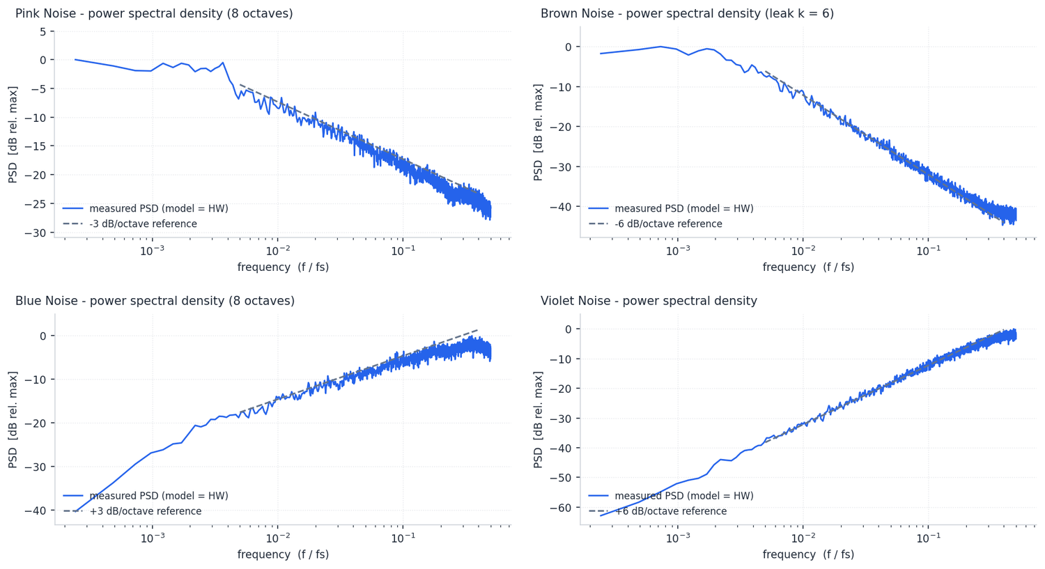
Those are the power spectral densities measured from the hardware model, each with its ideal slope drawn on top as a reference — which is the useful way to read them, because the interesting question about a noise block is not what it looks like but whether it lands on the law it claims.
Five shapes are available as separate blocks, and their implementations are worth knowing about because they explain why adding realistic noise costs almost nothing.
White is flat: the raw PRNG output. Pink, at −3 dB/octave, uses the Voss-McCartney algorithm — a set of octave registers refreshed at halving rates plus an always-new term, which is a handful of registers and one adder tree. Brown, at −6 dB/octave, is a leaky integrator on white, where the leak is what stops the DC drift and sets the low-frequency corner. Blue, at +3 dB/octave, is the first difference of pink, because differencing adds 6 dB/octave to whatever it is applied to. Violet, at +6, is the first difference of white.
None of them contains a multiplier or a block RAM. That is the point worth taking away: putting a physically realistic 1/f baseline into a test costs a few dozen flip-flops.
The one that matters most in practice is pink. Nearly every real analog front end has a 1/f component, from the preamplifier, from bias networks, from temperature. It is the disturbance that baseline restorers and DC blockers exist to handle, and it is the one that white noise does not exercise at all.
The distribution
Independently of the spectrum, the amplitudes can follow whatever shape the test needs.
Uniform comes from the PRNG directly, with the output width selectable from 2 to 64 bits and three algorithms to choose from: xoshiro256**, the Tausworthe LFSR258, and XorShift64. Triangular is the mean of two independent uniforms, signed and zero-centred, which costs one adder. Gaussian comes from the dedicated GNG block. Exponential is −ln(u), built from a count-leading-zeros, a log2 lookup and one constant multiply, with the mean landing exactly on 2^FractBits. Rayleigh is sqrt(−2 ln u), the same datapath plus an exact integer square root.

Three of them, measured over 131072 samples with the analytic density drawn on top. Note that the exponential is plotted on a log ordinate: what is being checked there is that the tail stays straight over four decades, which is where a cheap approximation would give itself away.
Exponential and Rayleigh are not exotic choices. Exponential is the distribution of intervals between Poisson events and of many first-passage times; Rayleigh is the envelope of a narrowband Gaussian process, which is what a magnitude detector downstream of a complex mixer actually sees.
And when none of the analytic shapes is right, Random Generator (Arbitrary Distribution) takes any distribution at all by inverse transform sampling from a CDF table, drawn in its designer from 58 built-in measured spectra, 20 analytic shapes, or an imported file. The programmable variant loads the table from a bus at runtime.
The arrival pattern
The third axis is when things happen. Poisson Pulser gives genuine Poisson arrivals with geometric inter-arrival times, at a rate that is a runtime pin. Periodic Pulse gives a strictly regular one. LFSR / PRBS gives a maximal-length pseudo-random sequence with a configurable register length from 3 to 64, both as a whole word and as the serial bit, which is what you need to exercise a serial link.
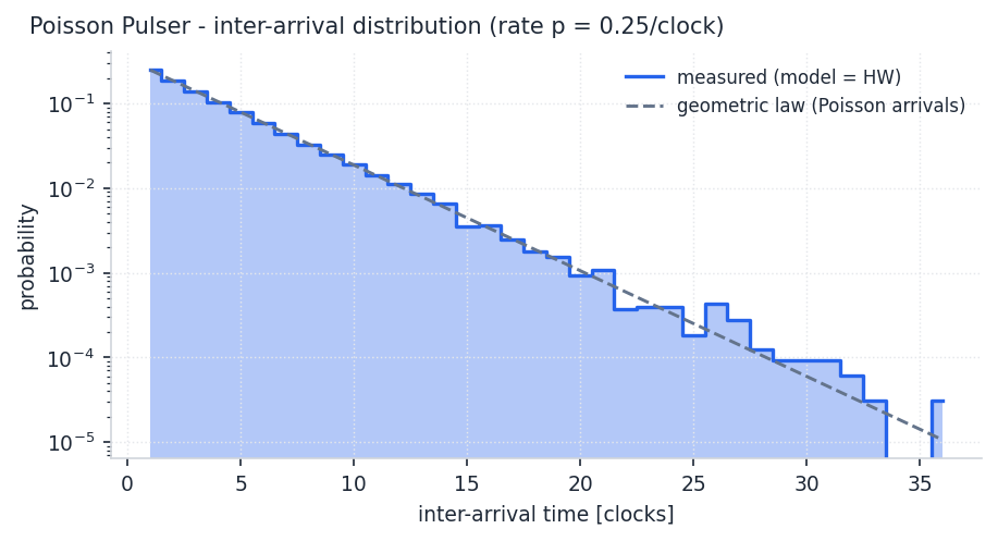
The distinction between “random” and “Poisson” is exactly the straight line in that plot. A pulse generator with a randomised period produces something that looks irregular; a Poisson process produces the geometric inter-arrival law, and that law is what determines how often two events land close enough together to pile up. If your rate test does not have this distribution, it is not measuring pile-up, it is measuring something adjacent to it.
The property that makes this a test rather than a demonstration
Every one of these blocks auto-randomises its seed when it is placed, so that two instances in the same design are independent rather than accidentally identical — which is a real trap, and one that produces mysteriously correlated “noise” on two channels.
But the seed stays editable, and RESET restarts the sequence identically.
That combination is what turns noise injection into a regression test. A run with a fixed seed is bit-for-bit reproducible, so a change in the output is a change in the design and nothing else. Without it, every comparison is confounded by the noise being different, and the only available conclusion is “roughly the same”, which is not a conclusion.
What it is worth doing with
Measuring a filter’s noise gain. Inject white noise of known variance, measure the variance out, compare against the theoretical gain of the coefficients. A discrepancy is a quantisation or saturation problem in the implementation, and it is invisible on a clean test signal.
Exercising a baseline restorer. Turn up the pink and brown components and watch how far the baseline moves. This is the test that the design was written for, and it is the test most often skipped because generating 1/f used to be awkward.
Characterising a trigger. Run a threshold against a known noise distribution and count the false triggers. Since the distribution is known exactly, the measured rate can be compared against the predicted one, and a mismatch means the threshold is not where you think it is.
Dither. A small triangular dither added before a quantiser decorrelates the quantisation error from the signal, turning a structured distortion into ordinary noise. Triangular is the right shape for this, and it is one block.
Monte Carlo in hardware. With arbitrary distributions available, a design can run a statistical simulation at the clock rate rather than in software.
The honest limitation
A synthetic noise source reproduces the statistics you asked for. It does not reproduce the noise of your particular front end, which has structure — mains harmonics, switching supply lines, digital crosstalk, microphonics — that no analytic distribution contains.
The right way to use these blocks is as a controlled, repeatable stress test of the digital chain, complementary to a measurement of the real thing. If you need to test against the real noise, capture it and replay it; if you need to test against noise you can specify, describe and reproduce exactly, generate it.
This is a reference design: the applications described are illustrative rather than an account of a deployed system. The spectra and distributions, however, are the blocks’ own characterisation figures, measured from the hardware model against the theoretical law.